An interactive graphical simulation of nucleic acid polymerases

Disclaimer: SimPol is currently in prerelease. It has not been peer-reviewed or published.

SimPol is a free open-source web-based program aimed to help researchers, teachers and students visualise transcription. Transcription is an essential pathway for all living organisms. It involves the copying of a template, typically DNA, into messenger RNA (mRNA) which is used to produce protein. Transcription is carried out by an enzyme called RNA polymerase. This webpage contains tutorials about SimPol and is hopefully friendly to all users.

Contents

Loading...


Getting Started


Information icons

Help icons are scattered throughout the interface of SimPol. Pressing one of these buttons will redirect to the relevant section on this page.

Conversely, there are direct links from this page to SimPol which look like this:     Example session: Open | View XML     The XML files that specify the session parameters can be downloaded or the session can be directly opened.


Sequence selection

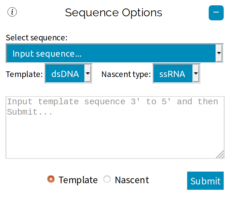
To enter a nucleic acid sequence, open up the ☰ Parameters side-navigation menu, under "Select sequence" choose "Input sequence", enter a sequence and then press Submit. A range of example sequences have also been provided. SimPol is designed primarily for transcription with DNA-dependent RNA-polymerases. The choice of template-type (DNA or RNA) and nascent-type (DNA or RNA) will dictate which thermodynamic parameters are used - Turner's RNA/RNA parameters, Sugimoto's DNA/RNA parameters, or SantaLucia's DNA/DNA parameters.


Polymerase structure

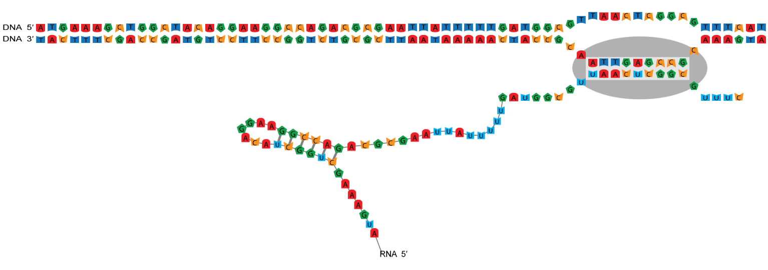
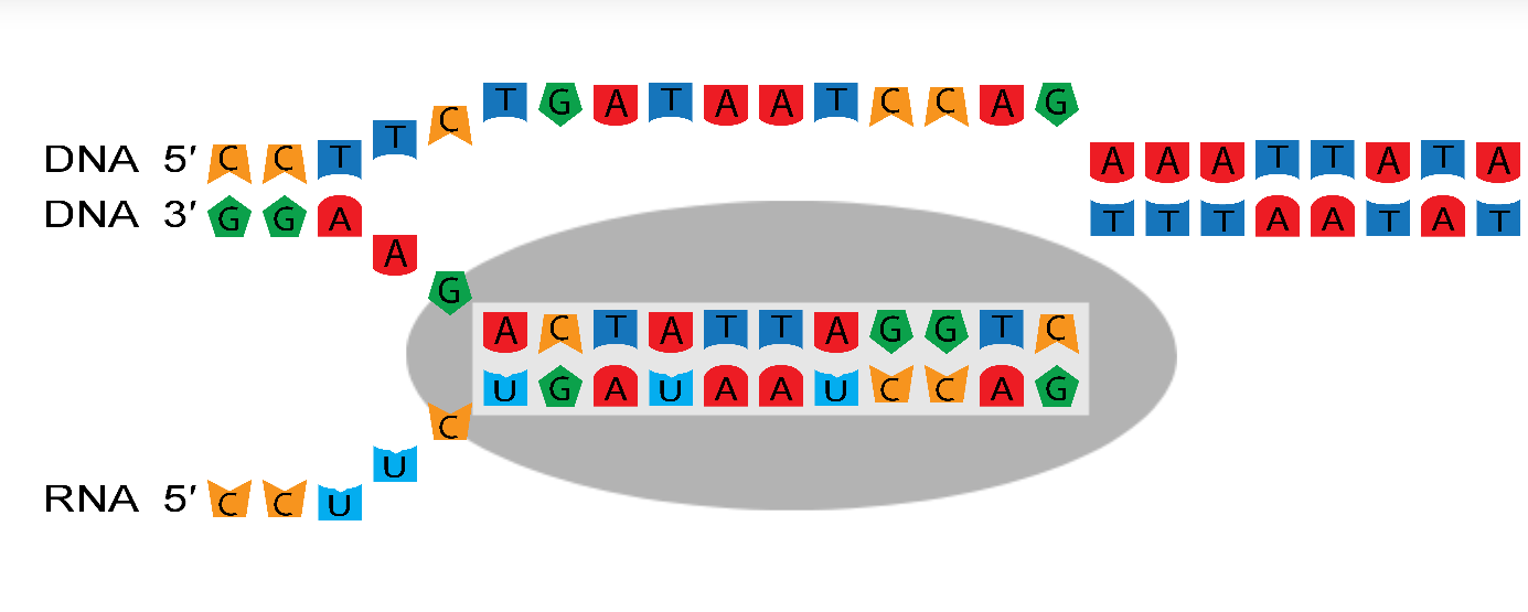
RNA polymerases reads the template strand (the gene) in the 3′ → 5′ direction, and copies it to create the nascent strand (the mRNA) which grows in the 5′ → 3′ direction. 
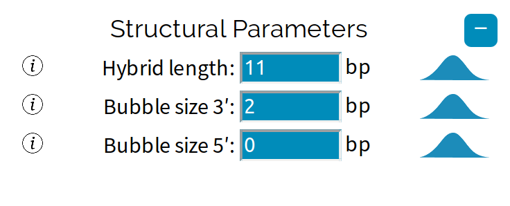
The transcription bubble consists of a hybrid between the nascent strand and the template strand within the polymerase, and a set of unpaired template bases upstream and downstream of the polymerase. In this example, the transcription bubble contains 2 + 11 + 0 = 13 bp.

The size of the transcription bubble differs between polymerases. These three parameters have a large effect on the sequence-dependent properties of the enzyme and can be changed from the ☰ Parameters side-navigation menu.


The toolbar

N =
The toolbar contains a range of essential functions.

Reinitiate resets the enzyme to its initial position. This will not affect plots or any other outputs. If any parameters have prior distributions then they will be resampled.

Stop immediately halts any polymerase acitivies taking place. This will not affect any parameters, plots or other outputs.

N = is a variable. The meaning of N depends on which tool is being used.

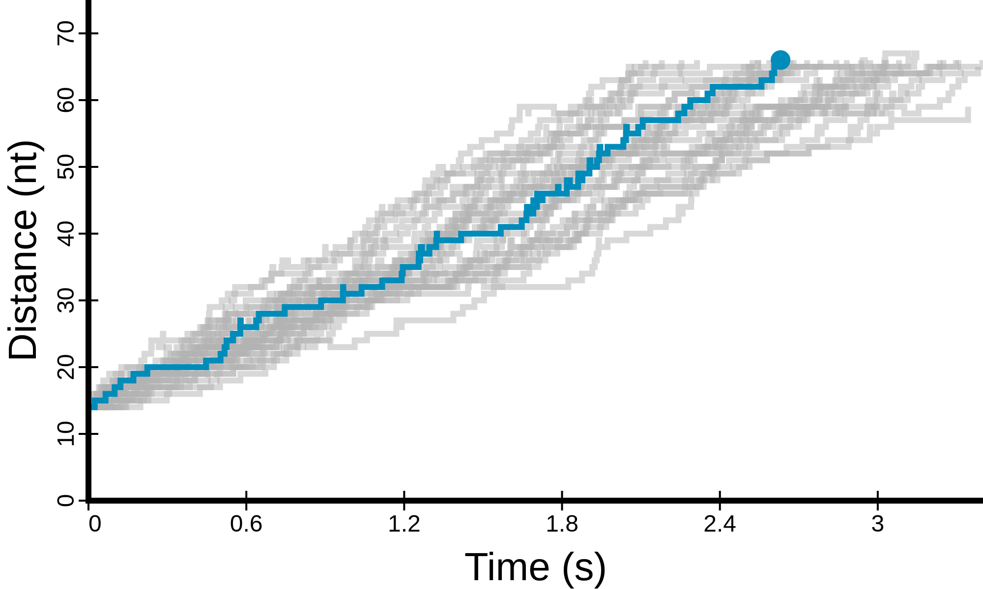
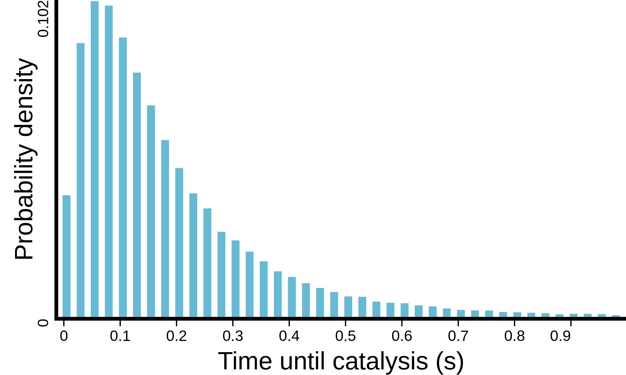
Simulate begins the random simulation starting from the current position of the polymerase. During the simulation, reactions are randomly sampled according to their rate constants, which can be tweaked in the parameters menu. N trials are performed in the simulation. When the polymerase finishes copying the sequence (or prematurely terminates) the next trial begins. The animation time of each reaction in the simulation is determined by Speed. The simulation can be stopped early using the Stop button.

Clear cache opens up a dialog to allow the deletion of any kinetic or sequence data which has been saved during the simulation. The kinetic data is displayed in plots so think of this button as resetting the plots.

Copy transcribes/replicates/copies the next N bases. The animation time is determined by Speed. Copying can be stopped early using the Stop button.

Stutter copies the current base N times, therefore adding an insertion of size N into the nascent strand. Insertions are added through slippage. The animation time is determined by Speed. Stuttering can be stopped early using the Stop button.

Fold folds the mRNA into its predicted secondary structure and renders the predicted structure. This function will only work if the nascent strand is single-stranded RNA. Note that this function is only cosmetic and will not affect the polymerase's kinetics. To incorporate mRNA secondary structure predictions into the kinetic model see . Folding is performed by the ViennaRNA suite.

Speed is a variable which controls the speed of the animation while Copying, Stuttering or Simulating. If the speed is set to slow, medium or fast, then the polymerase will animate each reaction at a slow, medium or fast speed, respectively. If the speed is hidden, then the polymerase is no longer displayed and will not animate at all. The plots will update periodically. Hidden is the fastest setting.

Save downloads the current session in XML format. If the page is refreshed or if your web browser crashes the settings will be lost.

Load uploads a saved XML session file.


States and Reactions


Kinetic model of transcription

Let $S(l,t)$ denote the current state, where $l$ is the length of the mRNA and $t$ is the position of the RNA polymerase (RNAP) active site with respect to the $3^\prime$ mRNA. Under the Brownian ratchet model, transcription elongation is a three step cycle. First, RNAP translocates from the pretranslocated position $S(l,0)$ into the posttranslocated position $S(l,1)$. Second, the incoming nucleoside triphosphate (NTP) binds to the active site of RNAP, $S_N(l,1)$. Finally, the bound NTP is incorporated onto the $3^\prime$ mRNA, returning the RNAP into the pretranslocated position $S(l+1,0)$.

However, RNAP does not always conform to this pathway. Periodically, RNAP backtracks ($t < 0$), whereby the enzyme translocates upstream causing the $3^\prime$ mRNA to exit through the NTP entry channel. This renders the enzyme catalytically inactive. It has been hypothesised that an intermediate state (IS) acts as a precursor for backtracking from the pretranslocated state. Alternatively, RNAP can hypertranslocate ($t>1$), whereby the enzyme translocates further downstream causing the shortening of the DNA/RNA hybrid.

Kinetic diagram
Hover over a state read its description.

In SimPol, backtracking, hypertranslocation, and the IS can each be enabled or disabled from the ☰ Parameters side-navigation menu. The kinetic diagram of the current model can be viewed using . Pressing the simulate button simulates the system according to the currently specified pathway. See Simulating.


Reactions

The polymerase can be controlled manually using the Navigation panel at the top of the main page.

Translocation: There are two translocation reactions: Backwards and Forwards. These operations move the polymerase one position left and right respectively, with respect to the template and nascent strand. These operations involve reconfiguring the base-pairs within the hybrid, and within the gene if it is double-stranded. If the polymerase moves beyond the 3′ end of the nascent strand (ie. hypertranslocation), then the nascent strand will be released (termination). Hotkeys: ← and → arrow keys
Nucleotide incorporation: If the active site is free and next to the 3′ end of the nascent strand, then the polymerase may bind NTP. Once bound, the polymerase may catalyse the reaction, or it may release the NTP back into the cell. Reverse-catalysis may also be performed (Lysis), although this reaction is often considered to be irreversible. The canonical pathway of transcription elongation is a three step cycle: 1) forward translocation, 2) NTP binding, 3) catalysis. This may also be achieved with the Copy function. Hotkeys: Shift + ← and → arrow keys
Inactivation: It is hypothesised that the catalytically inactive intermediate state, IS, acts as a precursor for backtracking. The Deactivate reaction causes the polymerase to enter the IS from the pretranslocated state, thus enabling backtracking to occur. The Activate reaction is the reverse.
Cleavage: When a nucleic acid polymerase backtracks for too long in vivo it can delay the production of its product and potentially cause roadblocks for other polymerases. Many organisms have evolved elongation factors which serve to rescue the polymerase from this state. One mechanism these factors may act is by cleaving the 3 end of the nascent strand when it pokes out the front of the polymerase during backtracking. This is carried out by GreA and GreB for prokaryotic RNA polymerases and S-II for eukaryotic RNA polymerase II and can be performed in SimPol using the cleavage reaction.
Slippage: During slippage, one strand in the (DNA/RNA) hybrid moves with respect to the other (ie. they slip along each other). Slippage is a key mechanism of insertion and deletion. In SimPol, this can be initialised using the Form Bulge reaction. When this happens, a nucleotide bulge forms within the duplex. This can occur within either the template or nascent strand (however in SimPol it can currently only occur within the nascent strand). When a bulge forms, the active site may be opened up, allowing one of the template bases to be copied twice. This would lead to an insertion. The bulge may diffuse left or right along the hybrid. This process is favoured if the hybrid sequence is repetitive (eg. AAAAAAAAA/UUUUUUUUU). When positioned at either end of the hybrid, the bulge may be absorbed. This three step process (bulge formation, diffusion and absorption) is based off the models proposed by Neher et al. and is believed to be the mechanism behind transcriptional slippage. Iterative slippage and elongation can lead to large insertions. This is sometimes called stuttering and can also be achieved with the Stutter function. Hotkeys: Ctrl + ← and → arrow keys


Plots
The output of the simulation can be visualised using various graphs, which are updated in real-time. These plots are displayed in the Plots panel and in the Sitewise panel. The display of each plot can be configured with its respective settings button. The raw data (.tsv) or a high resolution image (.png) can be downloaded . The different plots available are detailed below.
Distance vs time

This graph shows the progress made by the polymerase over time. The blue line represents the current simulation and the grey lines represent previous simulations. The x- and y-axis ranges can be set manually in the settings .
Time histogram

Depending on the settings , this will either show the total time taken to copy the template (one value per trial) or the time in between successive catalysis events.
Velocity histogram

These plots are histograms of the instantaneous velocities during elongation, as opposed to mean velocity. The instantaneous velocity at time $t$ is defined as the derivative of distance over time $v(t) = \frac{dx}{dt}$. However since the distance versus time function is discontinuous, there is no derivative. Instead, the instantaneous velocities are calculated as the mean velocities within non-overlapping fixed-sized windows. The window size parameter $w$ can be changed in the settings . The plots on the left illustrate the effect this parameter can have. Larger window sizes tend to underrepresent negative velocities, which correspond to net backwards translocation within the time window.
Parameter plot

Any parameter in the ☰ Parameters menu can be plotted onto this graph through the settings menu . The parameter's value will remain constant unless changed either (1) manually, or (2) by adding a prior distribution (see Adding a prior distribution to a parameter). Parameters are sampled from their prior distribution at the beginning of each simulation. Therefore one additional datapoint is made available to this plot at the end of each trial. Parameters can be compared with each other and with various measurements computed at the end of each simulation (mean velocity, mean catalysis time, mean total transcription time, and the final length of the nascent strand).

Elongation heatmap session: Open | View XML


Incorporation heatmap session: Open | View XML

Points can be coloured to represent a third variable, such as velocity. The third image shows the relationship between two parameters - and - required to achieve a velocity of 10-20 bp/s. As the rate of catalysis increases, the Gibbs energy barrier of translocation must increase with it in order to achieve the same velocity.

The forth images shows the relationship between and . As the dissociation constant of NTP binding increases, the concentration of NTP needed to achieve the same velocity increases.
MCMC trace

The trace plot is used to view the trace of an Markov chain Monte Carlo (MCMC) simulation (see MCMC-ABC). This is instrumental in interpreting chain convergence. The adjustable burn-in period is indicated by the red line. The variable displayed on the y-axis as well as the x- and y- axis limits can be adjusted in the settings . This plot is only accessible after MCMC has been initiated. Alternatively, the posterior distribution may be downloaded a as .log file and opened in Tracer.
Time per site

The time per site plots report the amount (or proportion) of time spent at each site in the template. Three options for the y-axis measure are available in the settings . First, the "Time to catalysis" of site $i$ is the mean time required to incorporate an NTP at site $i$, where the timer starts upon the incorporation of site $i-1$. Second, the "Time spent at site" of site $i$ is the mean time that the RNAP active site is positioned on $i$. This can illuminate where the RNAP is spending its time during backtracking. Third, the "Time per transcript length" of site $i$ is the mean time that the nascent strand has length $i$.


Parameters and Settings
Experimental Conditions
The concentrations of NTP (or dNTP if the nascent strand is DNA), and the size of the assisting force applied to the system

1 concentration 4 concentrations If this is set to 1 concentration then all four NTPs have the same concentration [NTP]. If this is set to 4 concentrations then the four NTP concentrations are set independently: [ATP], [CTP], [GTP], and [UTP]. Default: 1 concentration

[NTP] - concentration of all four NTPs (or dNTPs). Default: 1000 μM (or 20 μM)

[ATP] - concentration of ATP (or dATP). Default: 3152 μM (or 24 μM)

[CTP] - concentration of CTP (or dCTP). Default: 278 μM (or 29 μM)

[GTP] - concentration of GTP (or dGTP). Default: 468 μM (or 5.2 μM)

[UTP] - concentration of UTP (or dTTP). Default: 567 μM (or 37 μM)

$F_{assist}$ - the size of the force being applied to the polymerase during a single-molecule experiment. Positive forces are assisting loads and increase the rate of transcription. Negative forces are hindering loads and decrease the rate of transcription. In a natural cellular environment this external force is not applicable. Default: 0 pN

Halt - the position where the polymerase is halted prior to the start of the experiment. Change this value to start transcription further downstream. Default: 14 nt


Structural Parameters
Basepairing configuration within the transcription bubble and polymerase.

Hybrid length $h$ - number of basepairs in the template/nascent hybrid within the polymerase. As translocation rates are determined from sequence composition, this value may affect the predicted location of pause sites. Default: 11 bp

Bubble size 3′ $\beta_1$ - number of unpaired template bases 3′ (left hand side) of the hybrid. This parameter is only applicable if the template is double stranded. Default: 2 bp

Bubble size 5′ $\beta_2$ - number of unpaired template bases 5′ (right hand side) of the hybrid. This parameter is only applicable if the template is double stranded. Default: 0 bp


NTP Incorporation Parameters
Kinetics of binding/releasing NTP, and catalysing polymerisation.

Assume NTP binding equilibrium, $\mathbb{BE}$
If enabled, NTP binding is assumed to occur on such a rapid timescale that the NTP binding partial equilibrium assumption is applied. This will change how $K_D$ and $k_{bind}$ are interpreted. Default: true.

$K_D$ - equilibrium constant of NTP dissociation. If binding is assumed to be an equilibrium process ($ = 1$), $K_D$ is the ratio between the rates of NTP binding and release $K_D = \frac{k_{rel}}{k_{bind}}$. Whereas, in a kinetic binding model ($ = 0$) $K_D$ is used in conjunction with $k_{bind}$ to calculate the rate of releasing bound NTP: $k_{rel} = K_D k_{bind}$. Default: 97 μM

$k_{cat}$ - rate constant of incorporating bound NTP, thus extending the 3 end of the nascent chain by one nucleotide. When translocation is fast, catalysis is the rate limiting step in transcription. Default: 25 s-1

$k_{bind}$ - second order rate constant used to calculate rate constant of binding the complementary NTP, which is calculated as [NTP] kbind. If binding is assumed to be an equilibrium process ($ = 1$), this parameter has no meaning and the textbox will disappear. Default: 0.5448 μM-1.s-1


Translocation Parameters
Energetics of translocation reactions and force dependency.

Assume translocation equilibrium, $\mathbb{TE}$
If enabled, translocation between the pretranslocated and posttranslocated positions is assumed to be at equilibrium. Backtracking and hypertranslocation are not affected. This will change how $\Delta G^\dagger_\tau$ and $\delta_1$ are interpreted. Default: false.

$\Delta G^\dagger_{\tau}$ - Gibbs energy barrier of translocation. To translocate forwards or backwards, several basepairs may need to be broken. The energy barrier which must be overcome in order to translocate is estimated as the energy needed to break these basepairs plus the value of this parameter. Increasing this value will make translocation slower. When translocation is assumed to reach at equilibrium ($ = 1$), this parameter only applies to backtracking and hypertranslocation. Default: 5 kBT

$\Delta G_{\tau 1}$ - Gibbs energy term added to that of the posttranslocated state. When this value is low, RNA polymerase spends more time in the posttranslocated state (compared with the pretranslocated state). Default: -2 kBT

$\delta_1$ - position of the translocation transition state, compared with the two adjacent translocation positions. This parameter lies between 0 and the width of a single basepair in DNA (3.4 Å). This term only applies when translocation is kinetic ($ = 0$) and when an assisting force $F_{assist}$ is applied. Default: 3.25 Å

Transition state, $\mathbb{TS}$
A range of models for estimating the basepairing configuration of the translocation transition state. These models have a strong effect on the sequence dependent properties of the enzyme. See Kinetics of translocation. Default: HIGI model.


Pause Parameters
Kinetics of off-pathway translocation events.

Enable inactivation, $\mathbb{IS}$
If enabled, the intermediate state (IS) may be entered from the pretranslocated state. When enabled, this reaction is a necessary step for backtracking. Default: false.

$k_{U}$ - rate constant of polymerase entering the intermediate state. This state acts as a precursor for backtracking from the pretranslocated state. Default: 0.1 s-1

$k_{A}$ - rate constant of polymerase entering the pretranslocated state from the intermediate state. Default: 4 s-1

Enable backtracking, $\mathbb{BT}$
If enabled, the polymerase may backtrack. If the intermediate state is also enabled ($ = 1$), then entry into the intermediate state is necessary to begin backtracking. Default: false.

$\Delta G^\dagger_{\tau -}$ - Gibbs energy barrier of backtracking. To translocate forwards or backwards, several basepairs may need to be broken. The energy barrier which must be overcome in order to backtrack is estimated as the energy needed to break these basepairs plus $\Delta G_\tau^\dagger$ plus the value of this parameter. Increasing this value will make backtracking slower. Default: 0 kBT

Gating tyrosine, $\mathbb{GT}$
If this setting is enabled (-1 → -2 barrier), fast translocation between $S(l,0)$ and $S(l,-1)$ is permitted. Default: 0 → -1 barrier

Enable hypertranslocation, $\mathbb{HT}$
If enabled, the polymerase may hypertranslocate. This can lead to premature termination. Default: false.

$\Delta G^\dagger_{\tau +}$ - Gibbs energy barrier of hypertranslocation. To translocate forwards or backwards, several basepairs may need to be broken. The energy barrier which must be overcome in order to hypertranslocate is estimated as the energy needed to break these basepairs plus $\Delta G_\tau^\dagger$ plus the value of this parameter. Increasing this value will make hypertranslocation slower. Default: 0 kBT


RNA Folding Settings
Settings behind folding the nascent RNA strand.

$\lambda_b$ - the number of RNA nucleotides upstream and downstream from the polymerase which are sterically prohibited from folding. Default: 8 nt

Enable mRNA folding, $\mathbb{RB}$
If enabled, the nascent RNA strand will fold automatically during the simulation. The predicted energy barrier of unfolding secondary structures in the mRNA may need to be overcome when the polymerase translocates backwards. When the nascent strand is not ssRNA, this feature is not applicable. Note that enabling this option will slow down the first trial of the simulation as the secondary structure of the RNA is computed (MFE algorithm) using the ViennaRNA suite. You can view the RNA secondary structure with the Fold button. Default: false


Cleavage Parameters
Model for cleaving the nascent strand while backtracked.

$k_{cleave}$ - rate constant of cleaving the 3 end of the nascent strand when the polymerase is backtracked. In vivo this reaction may be carried out by elongation factors, for example, GreA. Default: 0s -1

$\lambda_{cleave}$ - the maximum number of positions that the polymerase may backtrack by in order for cleavage to occur. Set to 0 to have no upper limit. Default: 10 nt


Advanced Model Settings
Other parameters relating to the algorithm and model.

Arrest time - the amount of time the polymerase may take to termination before the simulation trial is aborted. When the timeout is reached, copying will prematurely terminate and the next trial will begin. Set to 0 to disable this feature. Default: 0 s

Proposal width - scale width of operators during MCMC-ABC search. Higher values result in larger steps and smaller values give smaller steps. Default: 1


Adding a prior distribution to a parameter


If uncertain about the value of a parameter, it can be given a background / prior distribution to capture its uncertainty. The probability distributions supported are uniform, normal, lognormal, and exponential. The parameter is resampled at the beginning of each simulation. All parameters are sampled independently of each other. This feature is useful for exploring the effect that parameters have on the system, or for fitting to a dataset.


Simulating


Equilibrium and the Boltzmann distribution

The Gibbs energy $G$ describes the work that can be performed by a thermodynamic system. The standard Gibbs energy of a reaction $\Delta G$ describes the change in Gibbs energy that accompanies a reaction of 1 M of reactants, under standard conditions (at 25°C and 100 kPa). $\Delta G_s$ describes how energetically favourable state $s$ is. A system spends more time in states which have low Gibbs energies. Suppose we have a single molecule which can exist in a number of chemical states. When the system has reached equilibrium, the probability of the molecule being in state $s$ at any given time is estimated with a Boltzmann distribution:

$$ p(s) \propto e^{-\frac{\Delta G_s}{k_B T}}, $$

where $\Delta G_s$ is the Gibbs energy of state $s$, $k_B$ is Boltzmann's constant ($1.3806 \times 10^{-23}$J.K$^{-1}$), and $T$ is the temperature in Kelvins. Energy is expressed in units of $k_B T$, by taking the experimental energy (in units of J) and dividing by $k_B T$.

For example, suppose a single molecule is in equilibrium between two states, $A$ and $B$. This is expressed as $A \rightleftharpoons B$. Suppose that the states have Gibbs energies of $\Delta G_A = -3\;k_B T$ and $\Delta G_B = -6\;k_B T$, respectively. We would therefore expect the molecule to be in state $A$ 4.7% of the time:

$$p(A) = \frac{e^{-\frac{\Delta G_A}{k_B T}}}{e^{-\frac{\Delta G_A}{k_B T}} + e^{-\frac{\Delta G_B}{k_B T}}} = \frac{e^{-\frac{-3\;k_B T}{k_B T}}}{e^{-\frac{-3\;k_B T}{k_B T}} + e^{-\frac{-6\;k_B T}{k_B T}}} = \frac{e^{3}}{e^{3} + e^{6}} = 0.047.$$


The Boltzmann distribution assumes that the system has been fluctuating for long enough to achieve equilibrium. However, since the competing processes of transcription (see Reactions) occur on similar timescales, equilibrium approximations do not always make good assumptions in this context.


Kinetics and the Arrhenius equation

Chemical kinetics is the study of rates of chemical processes, and how long reactions take to occur. A chemical reaction can be described with a rate constant $k$ (units s$^{-1}$). $k$ describes the speed of the reaction - a higher rate means that more reactions are expected to occur in a given time. Energy is required for a system to transit from one state to another. The standard Gibbs energy of activation for a reaction is denoted by $\Delta G^\dagger$. The larger this barrier, the more time needed for random thermal collisions to provide enough energy to allow the system to make the transition. Suppose a system is currently in state $s$, with Gibbs energy $\Delta G_s$. The Arrhenius equation can estimate the rate constant of transiting from state $s$ to state $s^\prime$:

$$ k_{s \rightarrow s^\prime} = A e^{-\frac{\Delta G^\dagger - \Delta G_s}{k_B T}}, $$

for some pre-exponential constant (units s$^{-1}$), where $\Delta G^\dagger$ is the absolute height of the Gibbs energy barrier between states $s$ and $s^\prime$. Once the rate constants of all possible reactions are known, we can start the single-molecule simulation.


The Gillespie algorithm

Transcription is simulated using the Gillespie algorithm. A critical assumption of this method is that these reactions are Poisson processes; the amount of time until a reaction occurs is independent of all other reactions and independent of the amount of time elapsed. For example, suppose we were to continue flipping a coin until it lands on tails. The probability of getting tails on the next flip is not affected by how many times we have already flipped, and is not affected by how many times someone else has flipped their coin. Similarly, whether a chemical reaction has been waiting 1 second or 1 hour for the reaction to occur, the probability of it happening right now is always the same. The amount of time until reaction $s \rightarrow s^\prime$ occurs follows the exponential distribution with rate $k$.

If there are multiple chemical reactions competing with each other, then the reaction with the shortest reaction time will be selected. For example, suppose we have have a test-tube containing a single molecule of compound $A$, which can spontaneously undergo two reactions: $A \rightarrow B$ or $A \rightarrow C$, with rate constants 0.001s-1 and 0.002s-1 respectively. The test-tube will flash a different colour of light for each reaction.

The amount of time until either one of these reactions occurs is random, and is exponentially distributed (see figure). If we were to simulate this on a computer, we could generate two exponential random variables, one from each distribution. For example, suppose we sampled time 769.14s for Exponential(0.001) and 339.81s for Exponential(0.002). Then reaction $A \rightarrow C$ would be selected because it has the shorter reaction time. The probability of sampling reaction $A \rightarrow B$ is

$$ p(A \rightarrow B) = \frac{0.001}{0.001 + 0.002} = 0.333,$$

and the probability of sampling reaction $A \rightarrow C$ is $0.667$.


Kinetics of nucleotide incorporation

Adding the next base onto the $3^\prime$ end of the nascent strand requires one translocation step (see Kinetics of translocation) and at least three chemical steps:

1. NTP binding. A free nucleoside triphosphate (NTP) molecule enters the active site and binds to the active site and its complementary base in the template.

2. Phosphodisester bond formation. The $5^\prime$ phosphate of thenucleoside monophosphate (NMP) is linked to the $3^\prime$-OH of the nascent strand.

3. Pyrophosphate release. The bound pyrophosphate is released back into solution.


Any of these steps could be reversible. As there is not sufficent information to model all three steps, nucleotide incorporation has been compressed into a two step process.

1. NTP binding. Step 1 from above. This is a reversible process. NTP binding/release is dictated by two parameters: and .

2. Catalysis. Steps 2-3 from above. This is assumed to be an irreversible process. The rate of incorporating a bound nucleotide is .


(units s$^{-1}$μM$^{-1}$) is the second order rate constant of binding NTP. The rate of binding an NTP is equal to $\times$ . Once the NTP has been bound, it may be released back into solution. The rate of release is calculated from the dissociation constant (units μM). Rate of NTP release is equal to $\times$ .

When the NTP concentration is high, or if is large, or if NTP binding is approximated as an equilibrium process ($ = 1$), then NTP binding becomes so rapid that equilibrium between these two states is achieved. Under these conditions, the kinetics of NTP binding are no longer relevant. is simply the ratio between the rates of binding and release, and can be used to calculate the proportion of time that NTP is bound. For example, suppose that = 35μM and = 1000μM, then the proportion of time that NTP is bound (while in this two-state system) is around 97%:

$$ p(\text{bound}) = \frac{ \frac{\text{[NTP]}}{K_D} }{\frac{\text{[NTP]}}{K_D} + 1} = \frac{ \frac{1000\text{ μM}}{35 \text{ μM}} }{\frac{1000\text{ μM}}{35 \text{ μM}} + 1} = 0.966. $$


Approximating NTP binding/release as an equilibrium process (using ) is equivalent to setting to a high value, however is much faster to simulate.


Kinetics of translocation

Let $\Delta G_{S}$ be the Gibbs energy of state $S$. In the context of nucleic acids, this can be approximated using nearest neighbour models. The basepairing energetic contribution of a transcription state is computed by summing the Gibbs energy of the gene to that of the hybrid:

$$ \Delta G_{total}^{(bp)} = \Delta G_{gene}^{(bp)} + \Delta G_{hybrid}^{(bp)} $$

Let $\Delta G_{S(l, t)}$ be the Gibbs energy of state $S(L, t)$. This term is calculated using:

$$ \Delta G_{S(l, t)} = \Delta G_{S(l, t)}^{(bp)} + \begin{cases} \Delta G_{\tau 1} &\text{ if } t = 1 \text { (posttranslocated) } \\ 0 &\text { if } t \neq 1 \end{cases} $$

where $\Delta G_{S(l, t)}^{(bp)}$ is computed from themodynamic parameters of nucleotide basepairing and is the Gibbs energy added onto the posttranslocated position.

If the rate of translocation is very rapid, or if translocation between the pre and posttranslocated states is approximated as an equilibrium process ($ = 1$), then these energetic terms describe the proportion of time the system spends in the two states. This is described by translocation equilibrium constant $K_\tau$.

$$ K_\tau = \frac{k_{S(l,1) \rightarrow S(l,0)}}{k_{S(l,0) \rightarrow S(l,1)}} = \frac{k_{bck}(S(l,1))}{k_{fwd}(S(l,0))} $$

However, in the general case, translocation is not assumed to reach equilibrium ($ = 0$). Basepairs may need to be broken in order for the polymerase to translocate forwards (right) or backwards (left) from its current position. For example, consider the state below.


For the polymerase to translocate one step backward, the doublet on the left of the transcription bubble and the doublet on the right of the hybrid must both be broken. For the polymerase to translocate one step forward, the doublet on the right of the transcription bubble and the doublet on the left of the hybrid must both be broken.

Let $S(l,t)$ and $S(l,t+1)$ be two neighbouring states and let $T(l,t)$ be the translocation transition state between the two. Using transition state theory, the Gibbs energy of this transition state is calculated as:

$$ \Delta G_{T(l, t)} = \Delta G_{T(l, t)}^{(bp)} + \Delta G_\tau^\dagger + \begin{cases} \Delta G_{\tau -}^\dagger &\text{ if } t \leq -1 \text{ (backtracking) }\\ 0 & \text { if } t = 0 \text{ (elongation) } \\ \Delta G_{\tau +}^\dagger &\text { if } t \geq 1 \text{ (hypertranslocation) } \end{cases} $$

where $\Delta G_{T(l, t)}^{(bp)}$ is the Gibbs energy of basepairing in the transition state, is the Gibbs energy barrier of translocation, is the Gibbs energy barrier of backtracking, and is the Gibbs energy barrier of hypertranslocation. Estimating $\Delta G_{T(l, t)}^{(bp)}$ can be achieved through several methods (discussed below). After the translocation energy barrier has been estimated, the rates of translocating between $S(l,t)$ and $S(l,t+1)$ can be calculated using the Arrhenius equation:

$$ k_{S(l,t) \rightarrow S(l,t+1)} = k_{fwd}(S(l,t)) = A e^{-(\Delta G_{T(l, t)} - \Delta G_{S(l, t)})} \\ k_{S(l,t+1) \rightarrow S(l,t)} = k_{bck}(S(l,t+1)) = A e^{-(\Delta G_{T(l, t)} - \Delta G_{S(l, t+1)})} $$

using pre-exponential constant $A = 10^6$ s-1.

SimPol has several methods for estimating $\Delta G_{T(l, t)}^{(bp)}$ (models are denoted by ):

i. Absolute model Translocation rates are determined exclusively from the energies of the translocation states and not the transition states. This is the simplest model, where

$$ \Delta G_{T(l, t)}^{(bp)} = 0. $$

ii. Midpoint model The Gibbs energy of basepairing of the transition state between $S(l,t)$ and $S(l,t+1)$ is calculated as

$$ \Delta G_{T(l, t)}^{(bp)} = \frac{\Delta G_{S(l,t)} + \Delta G_{S(l,t+1)}}{2}. $$

This was initially described by Tadigotla et al.
iii. Hybrid/bubble melting models Let $G$ be the set of basepairs within the gene of state $S(l, t)$, and let $G^\prime$ be that of $S(l, t+1)$. Similarly, let $H$ and $H^\prime$ be the sets of basepairs within the hybrid of $S(l, t)$ and $S(l, t+1)$ respectively. Then, the $H_IG_U$ model describes a transition state that is comprised of the intersection $\cap$ of the two hybrid basepairs sets, and the union $\cup$ of the two gene basepairs sets. Following this notation, there are four ways of directly evaluating $\Delta G_{T(l, t)}^{(bp)}$ using thermodynamic parameters:

$$ \Delta G_{T(l, t)}^{(bp)} = \begin{cases} \Delta G^{(bp)}(G \cap G^\prime, H \cap H^\prime) & \; \text{ if } \mathbb{TS} = H_IG_I \\ \Delta G^{(bp)}(G \cap G^\prime, H \cup H^\prime) & \; \text{ if } \mathbb{TS} = H_IG_U \\ \Delta G^{(bp)}(G \cup G^\prime, H \cap H^\prime) & \; \text{ if } \mathbb{TS} = H_UG_I \\ \Delta G^{(bp)}(G \cup G^\prime, H \cup H^\prime) & \; \text{ if } \mathbb{TS} = H_UG_U. \end{cases} $$

Here, $\Delta G^{(bp)}(x,y)$ denotes the Gibbs energy of a state comprised of a gene containing basepairs in set $x$ and a hybrid containing basepairs in set $y$. These four models describe physical mechanisms of translocation, each describing the ordering of basepairing melting and forming required to translocate.


In optical trapping experiments, beads are tethered to single molecules of RNA polymerase and optical tweezers are used to exert a force (units pN) upon the elongation complex. Positive forces $= F > 0$ act in the same direction as transcription (an assisting load) while negative forces $F < 0$ act in the opposite direction (a hindering load). Increasing the assisting force serves to decrease the Gibbs energy barrier of forward translocation and increase the barrier of backwards translocation. This process is modelled by adding an additional term to the Arrhenius equation:

$$ k_{fwd}(S(l,t)) = A e^{-(\Delta G_{T(l, t)} - \Delta G_{S(l, t)} - F(\delta_1))} \\ k_{bck}(S(l,t)) = A e^{-(\Delta G_{T(l, t-1)} - \Delta G_{S(l, t)} - F(\delta - \delta_1))} $$

where $\delta$ is the distance between consecutive basepairs ($\delta = 3.4$ Å in dsDNA), and 0 < < $\delta$ is the position of the transition state between the two neighbouring states.

The translocation equilibrium approximation asserts that is so small that translocation between the pretranslocated ($t=0$) and posttranslocated ($t=1$) states occurs on a timescale significantly faster than other reactions eg. NTP binding and incorporation.


Approximate Bayesian computation


Bayesian inference

Let $D$ be a dataset and let $\Theta = ${$\theta_1, \theta_2, \dotso, \theta_b$} be a set of parameters for a model. The goal of statistical inference is to find values for each parameter in $\Theta$ such that the model adequately describes the data $D$.

In Bayesian statistics, parameters are estimated using the posterior distribution. The posterior probability of $\Theta = \Theta_k$ can be obtained using: $$P(\Theta_k|D) = \frac{P(D|\Theta_k)P(\Theta_k)}{P(D)}$$ where $P(D|\Theta_k)$ is the likelihood - the probability of observing data $D$ under the model assuming that the parameters in $\Theta_k$ are set to their true values - and $P(\Theta_k)$ is the prior probability of $\Theta_k$ being the true values before observing new data $D$. $P(D)$ is a normalisation constant and is often intractable to evaluate directly. Subsequently, sampling methods are typically used to estimate the posterior distribution $P(\Theta|D)$. In a Bayesian framework, parameters are estimated as probability distributions - ie. the posterior distribution - instead of as point estimates.

Unfortunately, in some circumstances calculating the likelihood $P(D|\Theta)$ is not tractable. Instead, simulation can be used, and the posterior distribution can approximated. This framework is known as approximate Bayesian computation (ABC). Let $\rho(D,\hat{D}_k)$ be a function which evaluates the distance between the true data $D$ and the data $\hat{D}_k$ simulated under the model with parameters $\Theta_k$. Then, $\Theta = \Theta_k$ is accepted into the posterior distribution if $\rho(D,\hat{D}_k) \leq \epsilon$ for some threshold $\epsilon \geq 0$. The posterior distribution approximated under $\epsilon$ is denoted by $\hat{P}_\epsilon(\Theta_k|D)$.

If $\epsilon$ is sufficiently small, then $\hat{P}_\epsilon(\Theta_k|D)$ will be an accurate approximation of the true posterior distribution. However, if $\epsilon$ is too small, then adequately sampling from $\hat{P}_\epsilon(\Theta_k|D)$ may not be attainable in any reasonable timeframe.

In this section, first the various types of Experimental Data $D$ supported by SimPol are described. Then, two ABC algorithms for estimating $\hat{P}_\epsilon(\Theta_k|D)$ are explained: R-ABC and MCMC-ABC.
Experimental Data


SimPol supports three types of data, detailed below. The total experimental data is comprised of a series of $c$ experiments: $D = (d_1, d_2, \dotso, d_c)$. In the image above, there are $c=2$ experiments. Each datatype is associated with a distance function $\rho$. The values of $\rho$ (rho) are summed across each of the $c$ experiments to give the total distance.

Force-velocity data

In optical trapping experiments, varying forces are applied to the RNA polymerase using optical tweezers. As the assisting force increases, the rate of forward translocation increases with it.

Experimental dataset $d_i \in D$ consists of a set of experimental settings $F$ and observations $V$. $$d_i = \begin{bmatrix} F_i^1 & V_i^1 \\ F_i^2 & V_i^2 \\ F_i^3 & V_i^3 \\ \vdots & \vdots \end{bmatrix}$$ Vector $F$ describes the varying values of the applied Force used in the experiment. The NTP concentrations are held constant at specified values. The observations $V$ are the mean velocities of the polymerase, as measured under the applied force.

For force-velocity data, $\rho$ is the chi-squared statistic $X^2$: $$ \rho(d_i, \hat{d_i}) = X^2 = \sum_j \frac{(V_i^j - \hat{V}_j^j)^2}{\hat{V}_j^j} $$ where $V_i$ are the true velocities for experiment $i$, and $\hat{V}_i$ are the simulated velocities.


[NTP]-velocity data

By increasing the concentrations of the four NTPs, the elongation velocity is expected to increase with it.

Similar to force-velocity data, experimental dataset $d_i \in D$ is expressed as a matrix with experimental settings vector [NTP] and measurements $V$. For this data type, [NTP] describes the varying values of the NTP concentrations used in the experiment. Each NTP is associated with a concentration multiplier [ATP]eq, [CTP]eq, [GTP]eq, and [UTP]eq. The resulting concentrations for species _TP are computed as [NTP][_TP]eq. The applied force is held constant at a specified value. The observations $V$ are the velocities of the polymerase, as measured under the NTP concentrations.

For [NTP]-velocity data, $\rho$ is the chi-squared statistic $X^2$, calculated the same as for force-velocity data.


Pause site data

At a pause site, the polymerase takes significantly longer than average to incorporate the next nucleotide and move on to the next position.

When specifying pause site data, the indicies of all pause sites (defined as the length of the nascent strand when the pause occurs) must be indicated, and so must the full nascent sequence.

Let $f_P(j)$ describe the median time that nascent strand has length $j$, averaged across multiple simulations of the specified gene. SimPol treats pause site prediction as a binary classification problem. Subsequently, $\rho$ is equal to 1 minus the area under the curve (AUC) of a ROC curve, computed by comparing the known locations of pause sites with continuous function $f_P$. A single $\rho$ is computed across all pause site experimental datasets, as opposed to one per dataset as is the case in the previous data formats.


Motivating example 1

We will consider a simple example of using ABC to infer parameters of transcription elongation using a toy [NTP]-velocity dataset. The model assumes that NTP binding and translocation are at equilibrium and = 0. and are to be estimated and they have been assigned lognormal prior distributions. We will revisit this example using the R-ABC and MCMC-ABC algorithms.


For examples of ABC applied to real data, see SimPol in the Literature.


R-ABC

The rejection-ABC (R-ABC) algorithm is simple and easy to parallelise. Each sample is generated independently. The following user-specified settings are involved:
  • N iterations, $N$: the total number of samples from posterior distribution $\hat{P}_\epsilon(\Theta|D)$ to generate.
  • N trials per data point, $n$: the number of simulations per data point. The average measured value (mean velocity or median pause time) will be taken.
  • $\epsilon$: the threshold that $\rho(D,\hat{D}_k)$ must meet in order for $\Theta_k$ to be accepted into $\hat{P}_\epsilon(\Theta|D)$. This setting is linked with and can be used instead of $P(\rho \leq \epsilon)$.
  • $P(\rho \leq \epsilon)$: the probability that a value sampled from $P(\Theta)$ will be accepted. This setting is linked with and can be used instead of $\epsilon$.
  1. function R_ABC($D$, $\Theta$, $N$, $\epsilon$) {
  2.     $\hat{P}_\epsilon(\Theta|D) \leftarrow ${} // Initialise empty posterior distribution
  3.     for k = 1:N {
  4.         $\Theta_k \sim P(\Theta)$ // Sample $\Theta_k$ from prior distribution
  5.         $\hat{D}_k \sim $ simulator($\Theta_k$) // Simulate data using the parameters specified in $\Theta_k$
  6.         if ($\rho(D, \hat{D}_k) \leq \epsilon$) {
  7.             $\hat{P}_\epsilon(\Theta|D) \leftarrow \hat{P}_\epsilon(\Theta|D) \cup \Theta_k$ // Accept
  8.         }
  9.     }
  10.     return $\hat{P}_\epsilon(\Theta|D)$
  11. }

To test this algorithm on motivating example 1, follow the link below and then find and press . The posterior distribution can be summarised into a single state using .

R-ABC motivating example 1 session: Open | View XML


MCMC-ABC

The Markov chain Monte Carlo ABC (MCMC-ABC) algorithm produces a random walk through parameter space. Samples are no longer independent and therefore autocorrelation between successive states should be accounted for. In contrast to R-ABC, $\epsilon$ is not fixed. To enable $\rho$ to converge, $\epsilon$ starts out high at $\epsilon_0$ and then decreases to $\epsilon_{min}$ following an exponential cooling scheme: $\epsilon_i = \max(\epsilon_{min}, \gamma \epsilon_{i-1})$, where $0$ < $\gamma$ < $1$. $\epsilon_i$ refers to the value of the threshold at iteration $i$ in the MCMC chain. If $\gamma$ is too small, the system may not converge, whereas if $\gamma$ is too large then it may take too long to converge. The following user-specified settings are involved:
  • N iterations, $N$: the length of the chain of posterior distribution samples $\hat{P}_\epsilon(\Theta|D)$.
  • N trials per data point, $n$: the number of simulations per data point. The average measured value (mean velocity or median pause time) will be taken.
  • $\epsilon_{min}$: the final value of $\epsilon$ after cooling.
  • $\epsilon_{0}$: the initial value of $\epsilon$.
  • $\gamma$: the rate of $\epsilon$ cooling.
  • Burn-in (%): the percentage of samples to discard before reaching the posterior distribution. Set to -1 to allow automatic detection.
  • Log every (states), $L$: the frequency of storing posterior samples. Storing every sample is wasteful because of autocorrelation between successive samples.
  1. function MCMC_ABC($D$, $\Theta$, $N$, $\epsilon_0$, $\epsilon_{min}$, $\gamma$, $L$) {
  2.     $\Theta_0 \sim P(\Theta)$ // Initial state sampled from prior distribution
  3.     $\hat{P}_\epsilon(\Theta|D) \leftarrow ${$\Theta_0$} // Initialise posterior distribution
  4.     $\epsilon \leftarrow \epsilon_0$ // Initialise the value of $\epsilon$
  5.     for k = 1:N {
  6.         $\Theta^\prime \sim $ proposal$(\Theta_{k-1})$ // Sample proposal state using the proposal function. This randomly changes one parameter in $\Theta_{k-1}$.
  7.         $\hat{D}^\prime \sim $ simulator($\Theta^\prime$) // Simulate data using the parameters specified in $\Theta^\prime$
  8.         $\epsilon \leftarrow \max(\epsilon_{min}, \gamma \epsilon)$ // Lower the threshold
  9.         $u \leftarrow$ random_uniform(0,1) // A random number uniformly sampled from the range (0,1)
  10.         if ($\rho(D, \hat{D}^\prime) \leq \epsilon$ and $u$ > $\frac{P(\Theta^\prime)}{P(\Theta_{k-1})}$) { // Metropolis ratio
  11.             $\Theta_k \leftarrow \Theta^\prime$ // Accept
  12.         } else {
  13.             $\Theta_k \leftarrow \Theta_{k-1}$ // Reject
  14.         }
  15.         if ($k$ % $L$ = 0) {
  16.             $\hat{P}_\epsilon(\Theta|D) \leftarrow \hat{P}_\epsilon(\Theta|D) \cup \Theta_k$ // Log every $L$th state
  17.         }
  18.     }
  19.     return $\hat{P}_\epsilon(\Theta|D)$
  20. }

To test this algorithm on motivating example 1, follow the link below and then find and press . The posterior distribution can be summarised into a single state using . The chain is not guaranteed to converge and may tay a long time even if it does.

MCMC-ABC motivating example 1 session: Open | View XML


Model comparison
Recommended only for advanced users: the model itself can be estimated in Approximate Bayesian computation as well as the various Parameters. Kinetic models, which may differ in their model settings (for example equilibrium assumptions, whether backtracking is enabled) or by constraining parameters at fixed values, can be specified in the Model comparison panel. Prior probabilities may be assigned to each model by giving each model a weight. The probability that the model will be activated at the beginning of each simulation, or the prior probability of that model during approximate Bayesian computation, is proportional to that weight.

Upon pressing a new kinetic model will be created. The settings of that model will be those that are currently specified. Any parameters which do not have a prior distribution will be held fixed at their current value, and those which do have a prior distribution will be omitted from the model description. The model description can be manually edited.


Refer to SimPol in the Literature for real data examples of how model comparison has been used in inference.


Software Information


Running SimPol from the command line

The following instructions will work for Linux/Mac.
1. Generate a SimPol session file. Go to SimPol in your web browser and configure the number of trials, parameters, model settings, ABC settings, etc. When you are happy with all the settings, download the session as an XML file .

2. Download SimPol from here and unzip. Open up the command terminal and navigate to this folder.

3. Compile the ViennaRNA suite module. RNAfold is used when is enabled.

cd src/asm/ViennaRNA
bash build_vrna.sh

4. Compile SimPol. ViennaRNA must be successfully compiled first.

cd ../../../simpol/src/asm/
bash build_vrna.sh

5. Run SimPol.

bash simpol.sh -xml path/to/session.xml

where session.xml is the session generated earlier. This will run the number of simulations specified in the .xml file. Optional arguments:

-h: View the command line argument specifications.

-logO file.log: Write the MCMC-ABC or R-ABC output into the specified file.

-nthreads N: Parallelise the simulations over N threads. Multithreading does not work in the web browser, only from the command line. Default: 1.

-MCMC: Run MCMC-ABC analysis instead of simulating.

-resume: Resumes MCMC from the last state printed in the file specified by -logO and appends to -logO. Only applicable if -MCMC is enabled.

-logI file.log: Read in the specified file. Only applicable if either -summary or -RABC are activated.

-summary: prints a summary of the log file specified by -logI into the terminal.

-RABC: Run R-ABC analysis instead of simulating. All states will be printed regardless of the xml-specified value of epsilon. If -logI is specified then will sample from the posterior distribution, otherwise the prior. If -summary is also specified then will sample from the geometric median instead of the whole posterior distribution.


SimPol in the Literature


Bayesian inference and comparison of stochastic transcription elongation models

In this project (publication under review), we inferred kinetic parameters for three RNA polymerases: E. coli RNAP, S. cerevisiae pol II, and Bacteriophage T7 pol. The posterior distributions for these three experiments are available below. Posterior distributions may be viewed directly in the web browser or downloaded. Downloaded .log files can also be viewed with Tracer.

Enzyme View .xml Model Open Download .log


Jordan Douglas, Richard Kingston, and Alexei Drummond. "Bayesian inference and comparison of stochastic transcription elongation models." bioRxiv (2018): 499277. DOI: view


References


SimPol | Centre for Computational Evolution & School of Biological Sciences, University of Auckland | 2019